Abstract
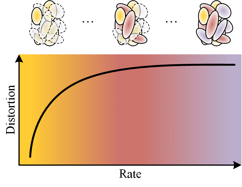
Recent advances in neural scene representations have transformed immersive multimedia, with 3D Gaussian Splatting (3DGS) enabling real-time photorealistic rendering. Despite its efficiency, 3DGS suffers from large memory requirements and costly training procedures, motivating efforts toward compression. Existing approaches, however, operate at fixed rates, limiting adaptability to varying bandwidth and device constraints. In this work, we propose a flexible compression scheme for 3DGS that supports interpolation at any rate between predefined bounds. Our method is computationally lightweight, requires no retraining for any rate, and preserves rendering quality across a broad range of operating points. Experiments demonstrate that the approach achieves efficient, high-quality compression while offering dynamic rate control, making it suitable for practical deployment in immersive applications.
Method Overview: Continuous-Rate 3DGS via Interpolation
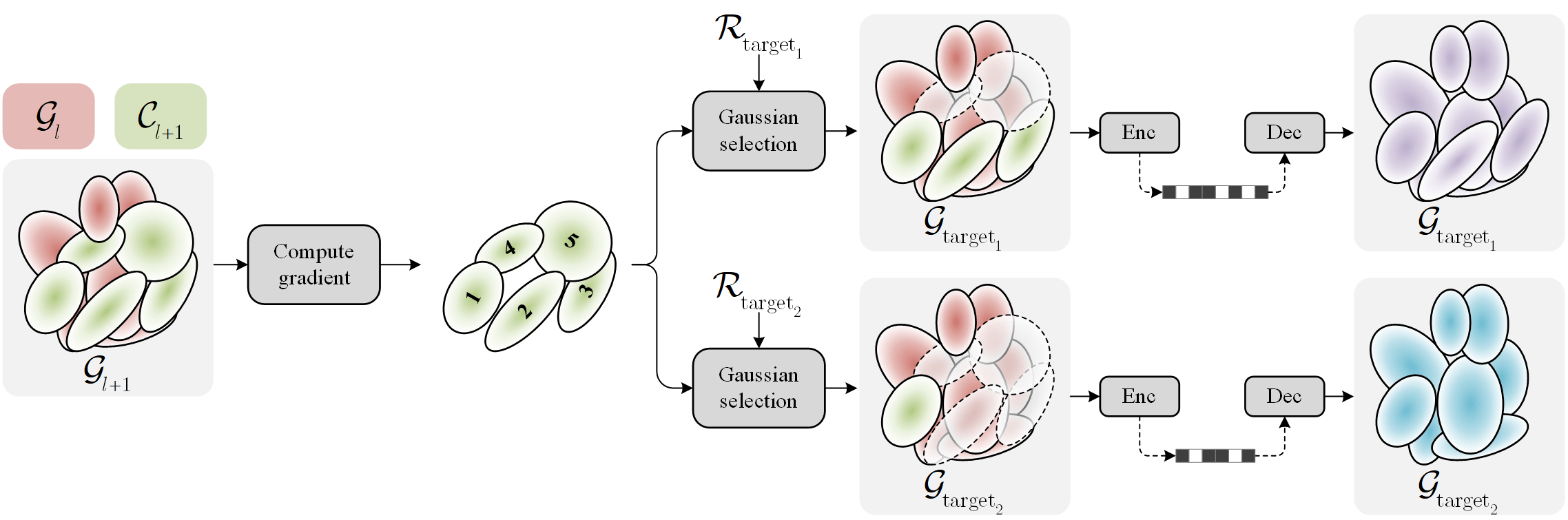
We compute per-anchor gradient scores once and rank Gaussians by importance. For any target rate \( \mathcal{R}_{\text{target}} \), the top-ranked Gaussians are selected to form \( \mathcal{G}_{\text{target}} \), then compressed and decoded to reconstruct the scene. This enables multiple operating points and a continuous rate–distortion curve from a single trained model.
Gaussian Selection
First, we train a scalable model by inheriting the ideas from levels of detail for 3DGS, GoDe. Starting from a pre-trained single-rate model (Scaffold-GS in our work), we divide Gaussians into \( L \) subsets according to a \( L \)-level progressive model. Formally, each level (anchor) is defined as \( \mathcal{G}_l = \bigcup_{i=1}^{l} \mathcal{C}_i \), with \( \mathcal{G}_l \) grouping Gaussians from the lowest rate anchor to \( l \), and \( \mathcal{C}_l \) representing our context comprising Gaussians to be introduced to move from anchor \( l-1 \) to \( l \). We perform quantization-aware fine-tuning to stochastically optimize all these anchor points.
Then, we can interpolate between any anchor pairs \( l \) and \( l + 1 \) by gathering all Gaussians from \( \mathcal{G}_l \) combined with a budget of most important Gaussians within the subset \( \mathcal{C}_{l + 1} \). This importance ranking is done by re-estimating the gradient w.r.t. the rendering loss. The number of Gaussians for a desired bitrate \( \mathcal{R}_{\text{target}} \) is:
\[ \left|\mathcal{G}_{\text{target}}\right| = \left|\mathcal{G}_{l}\right|+ \frac{\mathcal{R}_{\text{target}} - \mathcal{R}(\mathcal{G}_l)}{\mathcal{R}(\mathcal{G}_{l+1})-\mathcal{R}(\mathcal{G}_l)}(|\mathcal{G}_{l+1}| - |\mathcal{G}_l|) . \]
Among the budget \( |\Delta \mathcal{G}| = \left|\mathcal{G}_{\text{target}}\right| - \left|\mathcal{G}_{l}\right| \), we select the Gaussians having the highest gradient from the context \( \mathcal{C}_{l+1} \), assuming it is sorted by gradient:
\[ \Delta \mathcal{G} = \bigcup_{i=1}^{ |\Delta \mathcal{G}|}G_i \left|G_i\in \mathcal{C}_{l+1}, \left \lVert\frac{\partial \mathcal{L}}{\partial \theta_i} \right\rVert_2 \geq \left\lVert\frac{\partial \mathcal{L}}{\partial \theta_j} \right\rVert_2 \quad \forall i \in \{1, ..., |\Delta \mathcal{G}|\}, j \in \{|\Delta \mathcal{G}| + 1, ..., |\mathcal{C}_{l+1}|\} \right . , \]
where \( \theta \) represents the parameters of the Gaussian, and \( \mathcal{L} = (1 - \lambda) \mathcal{L}_1 + \lambda \mathcal{L}_\text{SSIM} \) is the standard rendering loss.
Note that our simple interpolation strategy is constrained to the granularity of a single Gaussian, but is compression backend-agnostic and can, in principle, be plugged into any compression pipeline.
Results


Mip-Nerf 360
Tanks&Temples
Deep Blending
Distortion-Rate comparison of our method (blue) against some SOTA methods: LightGaussian (purple), Reduced-3DGS (green), RDO (orange), and HAC (brown). Being the only continuous-rate method, our RD curves are indicated by a dense line ┃ instead of dotted line ┆ for other methods.


Mip-Nerf 360
Tanks&Temples
Deep Blending
FPS comparison of our method against the aforementioned SOTA methods.
Note that in Scaffold-GS representations, Gaussians are neural predicted using MLPs before
rendering. Hence, Scaffold-based methods (HAC and ours due to the selected backbone)
sacrifice significant rendering speed for compression rate.

Why context-aware pruning?
We compare our strategy (blue)
with a non-local variant (olive),
a naïve 50-level training (green),
and its variant in which the number of levels increases to \( |\mathcal{G}| \)
(orange).
The red anchor symbols ⚓︎ indicate the original anchors from which
we interpolate from.
Due to long-running time, this ablation is only conducted on the room scene.


Why ranking Gaussians using gradient?
We compare our selection criteria (blue)
with random selection (orange),
neural opacity-based ranking (purple),
neural size-based ranking (both bottom-up\( \nearrow \) green
and top-down\( \searrow \) lime, in which top smallest & largest
Gaussians are selected, respectively)
on the Mip-Nerf 360 dataset.
Illustrations
Bicycle
Bonsai
Counter
Flowers
Garden
Kitchen
Room
Stump
Treehill
Train
Truck
Drjohnson
Playroom
BibTeX
@misc{tran2025rave,
  title         = {RAVE: Rate-Adaptive Visual Encoding for 3D Gaussian Splatting},
  author        = {Hoang-Nhat Tran and Francesco Di Sario and Gabriele Spadaro and Giuseppe Valenzise and Enzo Tartaglione},
  year          = {2025},
  eprint        = {2512.07052},
  archivePrefix = {arXiv},
  primaryClass  = {cs.CV},
  url           = {https://arxiv.org/abs/2512.07052},
}